A method of modeling RF power amplifier circuit by using fuzzy neural network is proposed. Fuzzy neural network is a new type of network structure developed in recent years. It has the function of universal function approximator. The self-adaptive nerve in MATALAB is used in this paper. The fuzzy system ANFIS models the simulated data, and uses the obtained model to calculate the spectrum of the power amplifier, the power compression curve, the power gain curve, and the results of the ADS simulation, and obtains good results, which proves the modeling method. Effectiveness.
With the development of communication technology, RF circuits have been widely used in communication systems. The research and design of power amplifiers has always been an important issue in the development of communications. In recent years, the research on the modeling of RF devices and circuits based on fuzzy neural networks has achieved great results. It has great enlightening significance for the modeling of large-scale integrated circuits and complex circuits. It has become one of the hotspots of current research. This theory models and studies RF amplifiers.
1 Introduction to modeling methodsIn this paper, the first-order Sugeno model in fuzzy logic network is adopted. In order to realize the learning process of Sugeno fuzzy inference system, it is generally transformed into an adaptive network, namely adaptive fuzzy neural inference system, as shown in Figure 1.
The adaptive network is a multi-layer feedforward network, which can be divided into 5 layers, and the square nodes need to be parameterized. The following five layers are introduced separately.
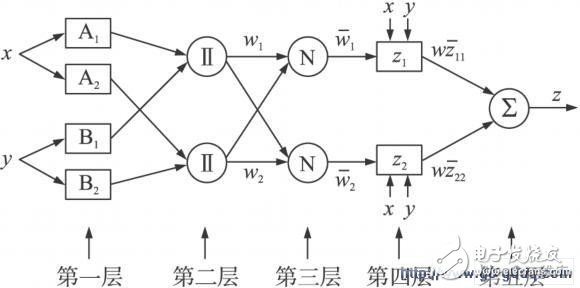
Figure 1 Structure of adaptive fuzzy neural inference system
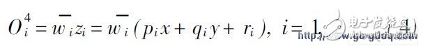
The first layer calculates the matching degree of the input variables, that is, the fuzzification process. Assuming that the fuzzy set uses a Gaussian function, then the layer output (Oi represents the ith output of the jth layer) is:
For the calculation of y, ci, σ i represent the center and width of the Gaussian function, respectively, which are parameters that need to be adjusted in the preconditions of the fuzzy rule.
The second layer calculates the excitation strength of the current input for each rule, and uses the membership of the fuzzy variables in the front part of the rule as a product, namely:
Layer 3 normalizes the excitation intensity:
The fourth layer calculates the output of each rule. The output of a rule is the product of the excitation strength of the rule and the conclusion part of the given input:
The fifth layer calculates the output of the fuzzy system, and the total output is the sum of all rule outputs:
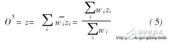
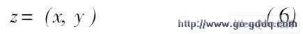
It can be seen that this fuzzy logic system defines a mapping from x, y to z:
By carefully selecting the parameters in the fuzzy rules, the relationship between the variables can be accurately characterized.
Modeling with fuzzy logic can divide the entire modeling process into two steps: the establishment of the initial model and the subsequent training adjustment of the model. In addition to the existing experience and knowledge in the field, the initial model can now be based on a set of training sample data, using a certain algorithm to determine the number of fuzzy sets of input variables and output variables and the corresponding membership function. Shape, and a set of fuzzy rules. With such an initial model, the learning algorithm, such as BP algorithm and DFP algorithm, is used to adjust the parameters in the membership function, and gradually reduce the error between the fuzzy output value of the system and the actual output value. Effect.
2 modeling processThe steps to apply ANFIS for modeling in the following examples are as follows:
(1) Simulate the designed power amplifier circuit in ADS. Here, the power amplifier circuits input as single tone signal, double tone signal and modulation signal are simulated respectively. The ultimate goal is to establish a behavior model describing the relationship between input and output ports. Therefore, the input and output voltage data are selected for training purposes.
(2) Write a program, preset the parameter values ​​in ANFIS, determine the type of membership function, the number of fuzzy rules, the number of iterations, the number of fuzzy sets, etc., establish an initial model, and complete the learning of training data; 3) Verify the model by using the sample data; adjust the parameters of the model by least squares and gradient descent.
(4) Observe the test result. If the test error meets the accuracy requirement, the modeling ends. If not, continue to adjust.
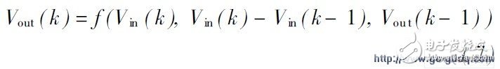
In this paper, an initial model of three-input and single-output is adopted. The input variables are selected as three input variables: Vin (k), Vin (k-1), and Vout (k-1), where Vin (k) is the input voltage and the variable Vin ( k - 1 ) is replaced by the differential form of Vin ( k - 1) = Vin ( k ) - Vin ( k - 1). Vout (k-1) is an item added in consideration of the memory effect, that is, the output of the previous moment. The output variable is a single variable Vou t ( k ). In this way, the dynamic relationship between the input and output of the entire circuit to be modeled can be expressed by equation (7):
The model adopts the Gaussian membership function, and the number of fuzzy rules is [2 12], a total of four, using the average segmentation method.
3 application examplesThe following is an RF power amplifier based on SM IC technology design, as shown in Figure 2. Its design indicators are as follows:
S11 " - 15 dB, S21" 20 dB, P1 dB 》 20 dBm, PAE 30%, PGAin 》 20 dB.
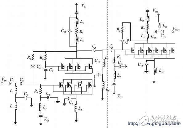
figure 2
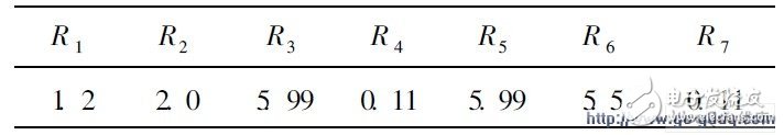
The N MOS tube in the SM IC library is selected in the circuit. The other component parameters are shown in Tables 1-3.
Table 1 Component parameter unit: pF
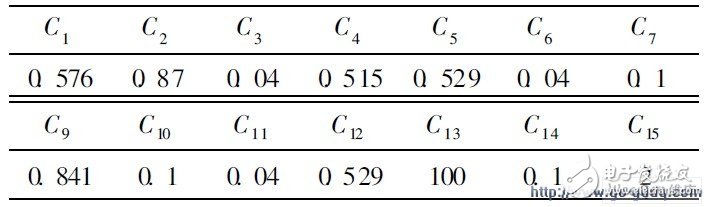
Table 2 Component parameter unit: nH
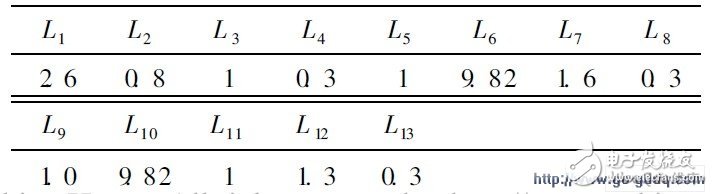
Table 3 Component parameter unit: kΩ
The circuit operates at 2.45 GHz, and the input power is RF_input= - 20 dBm~ 10 dBm (interval 1 dBm). The circuit is HB-simulated, and the sampling input and output voltage sampling data of two cycles in the time domain are selected. Training data. The selection of the test data is similar to the above, and one or more sets of signals within the input power RF_input= - 19. 5 dBm~1. 5 dBm (with an interval of 1 dBm) can be selected.
The modeling results are shown in Figures 3 to 6. Figure 3 shows the results of the steady-state output voltage at input powers of 6.5 dBm and - 6. 5 dBm.
Figure 4 shows the time domain data obtained by using the model with an input power of 7.5 dBm. The output voltage data of one cycle is selected for FFT transformation to obtain the spectrum of the voltage signal, and the power spectrum is calculated for the fundamental wave and the second to fifth harmonic voltages respectively. And compared with the spectrum obtained by ADS simulation. Figures 5 and 6 show the comparison of the power compression curve and the power gain curve calculated using the model data with the ADS simulation values.
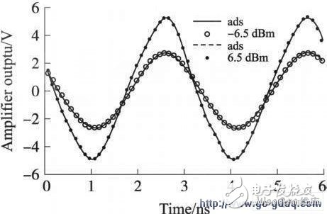
Figure 3 Steady-state output voltage curve
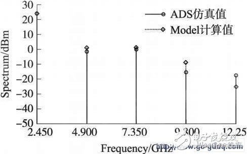
Figure 4 Comparison of model calculated values ​​and simulated values ​​of the spectrum
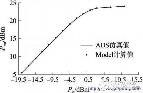
Figure 5 power compression curve
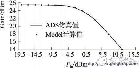
Figure 6 gain compression curve
As can be seen from the results in the figure, the results of the fuzzy logic model calculation are very good to the simulation results of the power amplifier circuit model.
The required output power and power gain can be obtained by the equations shown in equations (8) ~ (10):
Vout [1] is the fundamental term, sqr is the square function, mag is the function of the amplitude of the fundamental wave, the voltage is the peak value, so the square is divided by 2, the load is connected to 50Ω, and then the result calculated in parentheses is 10 The logarithm of the multiple is added to 30 and converted to an output power in dBm.
4 Conclusion
(1) In this paper, the fuzzy neural network structure is used to convert the data obtained by the power amplifier circuit through HB simulation into the time domain and establish a steady state model. The model calculates the spectrum characteristics, power compression characteristics and gain of the power amplifier in the frequency domain. The compression characteristics fully reflect the nonlinear characteristics of the supplier. The fundamental power calculated by the model fits well with the simulated value, and the power values ​​of other subharmonics are slightly different from the simulated values.
In addition, the circuit is modeled under the condition that the input signal is a two-tone signal and a modulated signal. The results of the model structure under these conditions are further analyzed. The results are basically satisfactory, but there are also a few points. Deviation, so the accuracy of the model has yet to be improved.
(2) Input the two-tone signal, perform two-tone balance simulation on the circuit, and observe the intermodulation distortion characteristics of the circuit. The input and output voltage data obtained by the dual-tone balance simulation are selected and modeled by the above model structure. The input powers P1 and P2 and the main frequency are changed to obtain 20 sets of input and output voltage values ​​as training data. P1 and P2, - 24~ - 20dBm, interval 1 dBm; main frequency selection 2 45 GHz and 2 25 GHz.
The test data is selected at 2 45 GHz, P1 - 19 dBm, P2 - 23dBm input and output voltage data. The modeling results are shown in Figure 7. It is known that (the dotted line represents the calculated value of the model and the solid line represents the actual simulated value). The effect of the model fitting is good.
(3) Using the CDMA modulation signal source in the ADS simulation circuit, adding a modulation signal to the power amplifier circuit, performing envelope simulation, and extracting information of the input signal and the output signals Rea l part and Im part. By changing the power of the input signal, 10 sets of input and output Rea l part data are obtained as training data (-9-9 dBm, interval 2 dBm), and each set of training data is sampled by 300 points. The test data is selected from a set of data with an input power of 4.5 dBm. Modeled using the above method, the results are shown in Figure 8. Similarly, data of 10 sets of Im part can be extracted as training data for modeling, and the result is shown in FIG. 9. By comparison, the calculated results of the model are basically consistent with the actual values, and there are a few points where deviations occur.
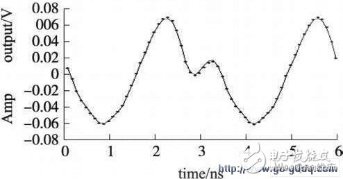
Figure 7 Circuit output waveform under two-tone signal input condition
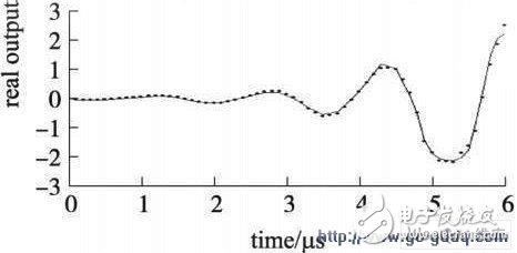
Figure 8 Input power 4. 5 dBm output real waveform
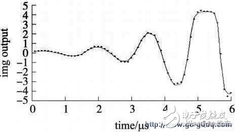
Figure 9 Input power 4. 5 dBm output imaginary waveform
Firewall Pc With Tpm,Firewall Router With Tpm,Pfsense Firewall With Tpm,Network Server With Tpm
Shenzhen Innovative Cloud Computer Co., Ltd , https://www.xcypc.com